Radar Recollections - A Bournemouth University / CHiDE / HLF project

Radar from little acorns - A short primer in Radar Theory

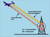If a reflective object (such as an aeroplane) obstructs this radiation, most will be absorbed but a small proportion will be reflected back to the source. So the distance to the object [d] means that the returned beam will have traveled 2d. The time taken [t] for the beam to make this journey will be: t = 2d / c.

'Time' is the easiest of all physical variables to measure accurately.

More useful is the formula: d = tc / 2 because this gives us the distance that the object is from the transmitter. It is also important to know the horizontal (azimuth) bearing that the reflected signal in returning from. The design and directional
capabilities of both transmitting and receiving aerials will determine the accuracy and precision of the instrument.

Height determination is more complex and involves assessing the 'angle of elevation'. Essentially, two aerials, transmitting beams pointing up at different angles will give slightly different lengths for the reflected signal and will return at different times. These time differences can be measured. Triangular geometry will do the rest.

Early directional radar depended on at least two receiving aerials spaced up to one km apart and then measuring the time difference between the signal returning to each aerial. Directional aerials soon became augmented with rotational ones. The size of the antenna required is proportional to the wavelength chosen for transmission, so the longer the wavelength, the larger the aerial.

At long wavelengths (eg. 50 metres) only large objects will reflect back a complete radiation pattern for collection. Therefore, if small objects (such as a fighter plane) need to be accurately recorded, much shorter wavelengths must be employed. Atmospheric interference is also less pronounced at shorter wavelengths.

TOP OF PAGE

So why was it not possible to use shorter wavelengths to begin with?

Until the Autumn of 1940, the transmitters that were being produced were not sufficiently advanced enough to work effectively at centimetric wavelengths. They were capable of generating considerable power outputs, but only for longer wavelengths. Although refinements to the circuits (particularly using the Klystron) gradually added to the outputs obtainable, there was a functional limit at about 1.5m wavelength. A power increase of 10 was required. This was only made possible with the introduction of the Cavity Magnetron in 1940.

TOP OF PAGE

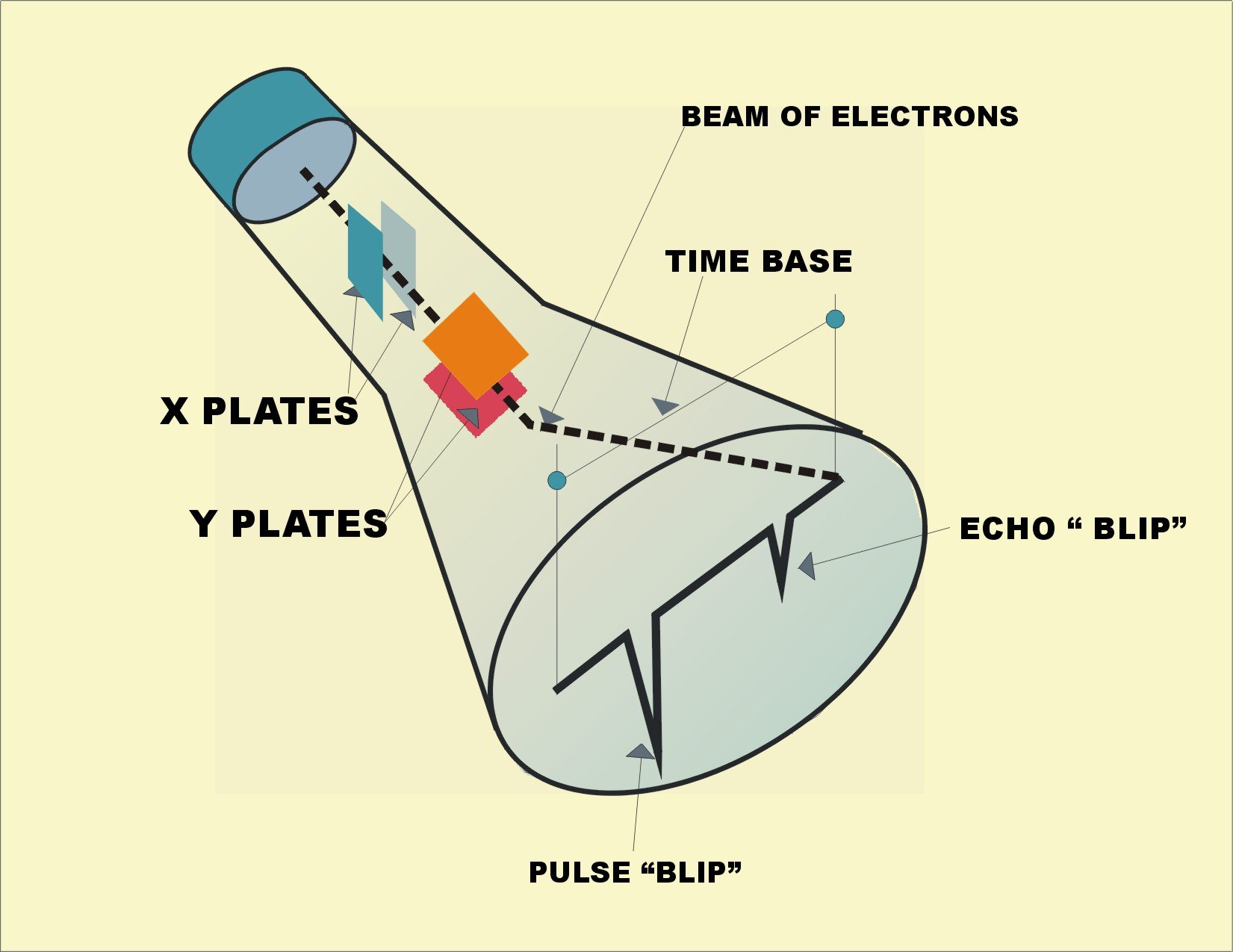
Another problem is that transmitting a continuous wave would mean that a continuous 'medley' of incoming signals would be received. The answer was to 'pulse' the waves out at a known frequency and then each returning signal could be electronically 'matched' to its outgoing parent wave. Eventually it was possible to develop systems that used a combined Transmitter (Tx) / Receiver (Rx) aerial by switching the array many times a second from Rx to Tx in synchrony. This timing can be controlled and locked. The manifestations of these signals can be observed when the Tx and Rx signals are fed into a Cathode Ray Tube Oscilloscope….

TOP OF PAGE

An electron beam is focused to run from 'A' to 'B' in a regular and precise fashion and constitutes the 'timebase'. An incoming signal will interrupt the regular movement of electrons because the new signal will slightly alter the voltage across the 'Y' plates and hence deflect the beam. The stronger the signal, the greater the voltage disruption and the greater the electron deflection. The whole process can now be displayed visually on the oscilloscope. The range of the object from the transmitter will always be a function of the distance between the outgoing pulse 'blip' and the (much weaker) incoming echo 'blip. The further apart the two 'blips' appear on the screen; the further away the object actually is. By calibrating the timebase [AB] (in miles), it is possible to estimate the true distance of the object.

TOP OF PAGE

Contents page
Home page